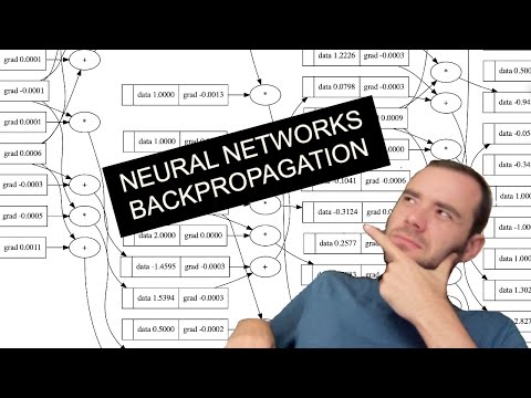
The Spelled-Out Intro to Neural Networks — Andrej Karpathy
“This is hands-down the single best tutorial on backprop and computational graphs on the entire internet. He codes up an autograd engine from scratch with zero magic.”
Executive Summary: Spelled-Out Intro to Neural Networks and micrograd
A bottom-up, zero-magic reconstruction of backpropagation and deep neural networks foundations from Andrej Karpathy’s renowned “Neural Networks: Zero to Hero” lecture series. Karpathy builds micrograd—a minimalist scalar autograd engine—in approximately 100 lines of pure Python, demonstrating that modern deep learning frameworks like PyTorch are fundamentally orchestration layers around computational directed acyclic graphs (DAGs) and calculus chain rule accumulators. This spelled-out intro to neural networks explains how scalar values, forward computation graphs, and reverse topological gradient backpropagation cooperate to train neural networks without high-level library black boxes.
Key Mental Models Derived from this Lecture:
- The Computational Graph as a directed acyclic graph (DAG) where nodes are scalar Values and edges are mathematical operations (+, *, tanh).
- Local Gradients and Calculus Chain Rule: Every arithmetic primitive knows how to compute its local partial derivative with respect to its immediate parents.
- Global Derivative Accumulation: Backpropagation in neural networks is reverse topological sorting over the DAG, multiplying local derivatives along path branches.
- Gradient Accumulation (+=): Crucial insight: gradients must accumulate with += rather than assignment (=) to handle multi-variable reuse and multi-path graph flow correctly.
- Loss Function and Optimization Step: Mean Squared Error (MSE) loss quantifies network error, and stochastic gradient descent iteratively nudges scalar weights opposite to their gradient directions.
- From Scalar Autograd to Tensor Networks: Understanding micrograd demystifies how PyTorch tensors parallelize identical scalar graph rules across GPU matrix multiply CUDA kernels.
Key Timestamps: Spelled-Out Neural Networks Lecture Breakdown
Derivative Intuition via Infinitesimals in Neural Networks
The Value Class: Building the Computational Graph DAG
Manual Backpropagation on a Single Neuron Architecture
Automating Reverse Topological Sort for Backpropagation
Building Neuron, Layer, and MLP Multi-Layer Perceptron Containers
Training a 2-Layer Neural Network and Debugging Gradients
Mathematical Derivations: Backpropagation in Neural Networks
Scalar Chain Rule (Calculus Foundation of Neural Networks)
If variable z depends on y, and y depends on x, the rate of change of z with respect to x is the product of their local rates. In backpropagation, upstream gradient times local derivative yields the upstream sensitivity.
# Backward step for multiplication: out = x * y
def _backward():
    self.grad += other.data * out.grad
    other.grad += self.data * out.grad
Tanh Activation Derivative in Backpropagation
Crucial efficiency trick: once the forward output t = tanh(x) is cached, the backward pass only requires 1 - t^2, avoiding recomputing expensive exponentials during neural network training.
t = self.data
self.grad += (1.0 - t**2) * out.grad
Mean Squared Error (MSE) Loss Derivative
The objective function quantifies prediction error across training examples. Differentiating MSE with respect to predictions initiates the backward pass with the initial error vector.
loss = sum((yout - ygt)**2 for ygt, yout in zip(ys, ypred))
loss.backward()
Multi-Path Gradient Summation (Multivariate Chain Rule)
When an intermediate variable is reused across multiple computational graph branches, its total derivative is the sum of partial derivatives flowing through every individual path.
# Must use += instead of = to accumulate gradients across multiple branches
self.grad += local_derivative * out.grad
Parameter Update Step (Stochastic Gradient Descent in Neural Networks)
Subtracting the gradient steps parameters in the direction of steepest loss descent. Crucially, parameter gradients must be reset to zero before the next forward-backward iteration.
for p in model.parameters():
    p.data -= learning_rate * p.grad
p.grad = 0.0 # Reset gradient buffer for next stepCommunity Consensus: Hacker News Debates on Neural Networks and micrograd
Scalar Autograd vs. Tensor PyTorch Memory Overhead
“The moment you understand micrograd, the mystique of PyTorch vanishes. It proves autograd is just topological sort plus chain rule.” — @dr_krapf
The += vs = Gradient Accumulation Bug Trap in Backpropagation
“Multivariate chain rule requires summing over all paths. Andrej highlighting the bug where a node is used twice was worth watching the entire 2 hours.” — @eigen_state
Karpathy’s Neural Networks: Zero to Hero vs Traditional University Curriculums
“Andrej’s teaching method turns the deep learning black box into glass. You realize a neural network is not magic, it’s literally just chained arithmetic with gradient tape.” — @vector_field
A Recipe for Training Neural Networks: Andrej Karpathy’s Debugging Philosophy
“Karpathy’s golden rule of neural networks: do not look at hyperparameters until you have visually verified your gradients and overfit one batch. That single discipline saves weeks.” — @loss_divergence
Technical FAQ: Neural Networks, Backpropagation and Training Recipe
In Simple Made Easy, what is the fundamental difference between Simple and Easy?
In the Simple Made Easy lecture by Rich Hickey, Simple is an objective design property (simplex: having a single role, unbraided), whereas Easy is subjective and relative to developer familiarity (facilis: near at hand).
What does the Simple Made Easy lecture mean by the verb “to complect”?
In Simple Made Easy, to complect means to braid, intertwine, or fold multiple distinct concerns together (from Latin complecti). Once concepts are complected, you cannot reason about or test one without dragging the other along.
Why does Simple Made Easy advocate for immutable values over mutable state?
Simple Made Easy proves that mutable state braids value and time together. Immutable values represent permanent historical facts that can be freely shared across concurrent threads without locks, cached indefinitely, and trivially reasoned about.
How does the Epochal Time Model in Simple Made Easy solve concurrency?
In Simple Made Easy, identity is an atomic reference pointing to an immutable value snapshot at time t. Updates apply a pure function to produce a new immutable value at t+1 and swap the reference atomically (e.g. CAS), allowing lock-free reads.
Why does Simple Made Easy recommend passing plain data maps instead of OOP classes?
In Simple Made Easy, plain associative maps represent information directly without braiding data representation with domain logic or class inheritance hierarchies, enabling universal composition.
What architectural constructs does Simple Made Easy recommend for decoupled systems?
Simple Made Easy recommends five foundational constructs: persistent immutable data structures, declarative data (like JSON or EDN), asynchronous queues to decouple space and time, pure functions, and runtime schemas.